Principles of Microeconomics

MIT OCW 14.01SC - Summary

Economics is about scarcity and resource optimisation.
Microeconomics tries to model a general decision making framework.
We look at behaviour of two main actors in Microeconomics: Producers and Consumers.
One key variable: Prices. Prices determine resource production, consumption and allocation.
Positive vs Normative economics: How things are? vs How things should be?

Supply and Demand curves. Equilibrium point at intersection.
- Q_d = D(P)
- dQ_d / dP < 0 (Law of Demand)
- Q_s = S(P)
- dQ_s / dP > 0 (Law of Supply)
- Q_d (P*) = Q_s (P*)
- P* is optimal price.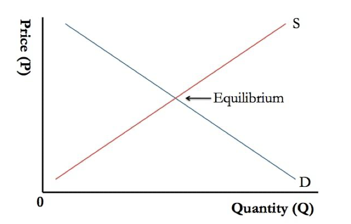
Supply and Demand curve shifts due to shocks
- Market absorbs excess supply and excess demand by shifting equilibrium.
- Price changes in one market can affect another.
  - General equilibrium includes feedback effects.
Government Intervention in Markets.
- Eg. Minimum wage, Price ceilings.
- May cause inefficiences, e.g. unemployment, shortages.
- Equity-Efficiency tradeoffs.
  - Costs:
    - Efficiency loss - trade that could make both parties better off is not made.
    - Allocation inefficiency - resources are not allocated to those who need them the most.
  - Benefit:
    - Equity - (percieved?) fairness.
- Direct effects (what voters see) and indirect effects (what economists see).
- Secondary markets can arise to evade government regulation.

Elasiticity of demand (\epsilon_d) = (dQ/Q)/(dP/P) = (dQ/dP)*(P/Q). (units: dimensionless, ratio of %s) (should be negative) (percent change in qty / percent change in price)
- Perfectly Inelastic Demand: elasticity = 0.
- Perfectly Elastic Demand: elasticity = -infinite.
Perfectly Inelastic Demand
- Demand does not change with price change
- Straight vertical line on price-qty diagram.
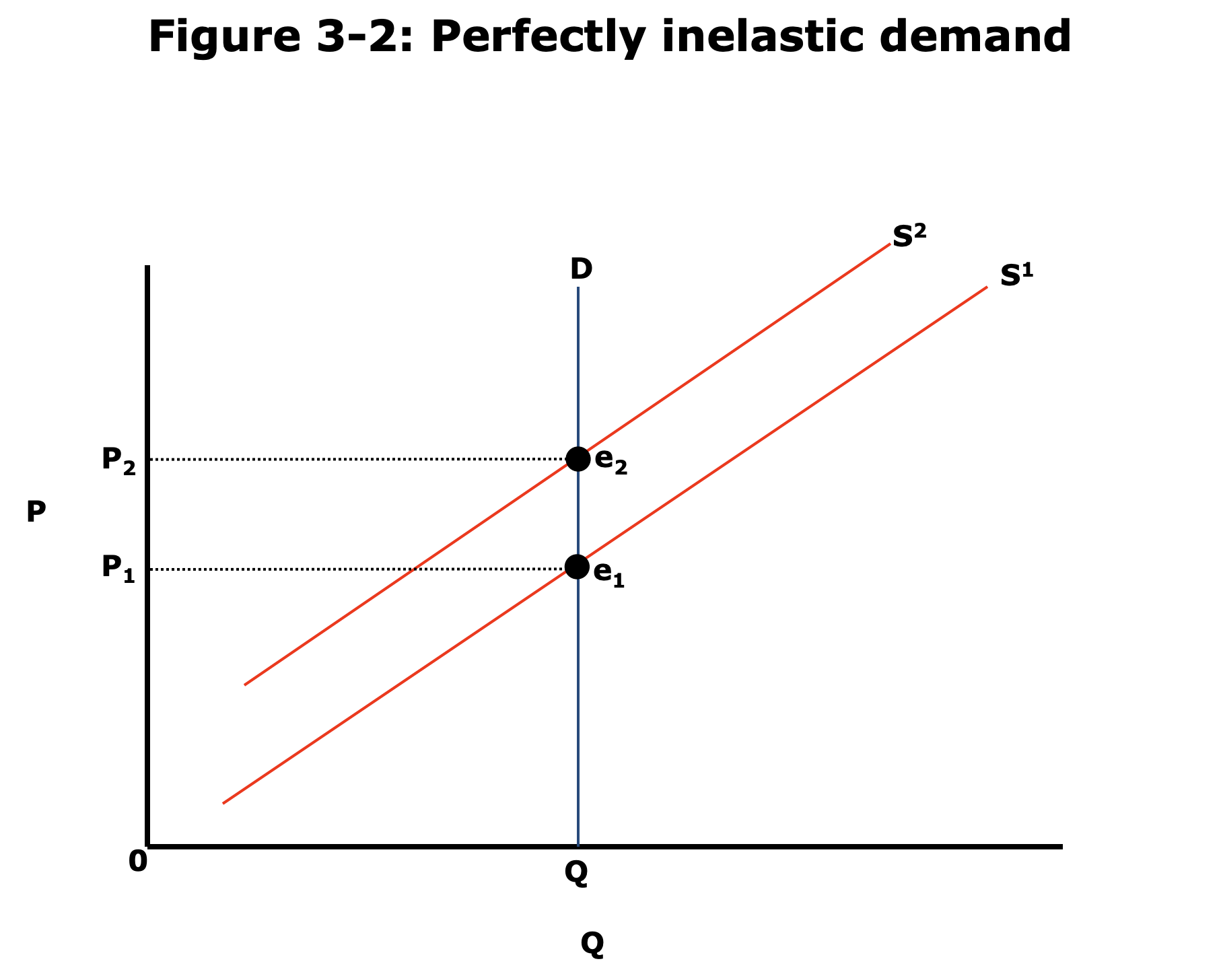
- Example: when there are no substitutes.
  - Some Medicine / treatments - e.g. insulin for diabetics.
  - Example of elastic demand: viagra.
- What happens in case of supply shock?
  - If supply decreases(?) There cannot be excess demand. The price increases. No change in qty.
Perfectly Elastic Demand.
- Straight horizontal line on price-qty diagram.
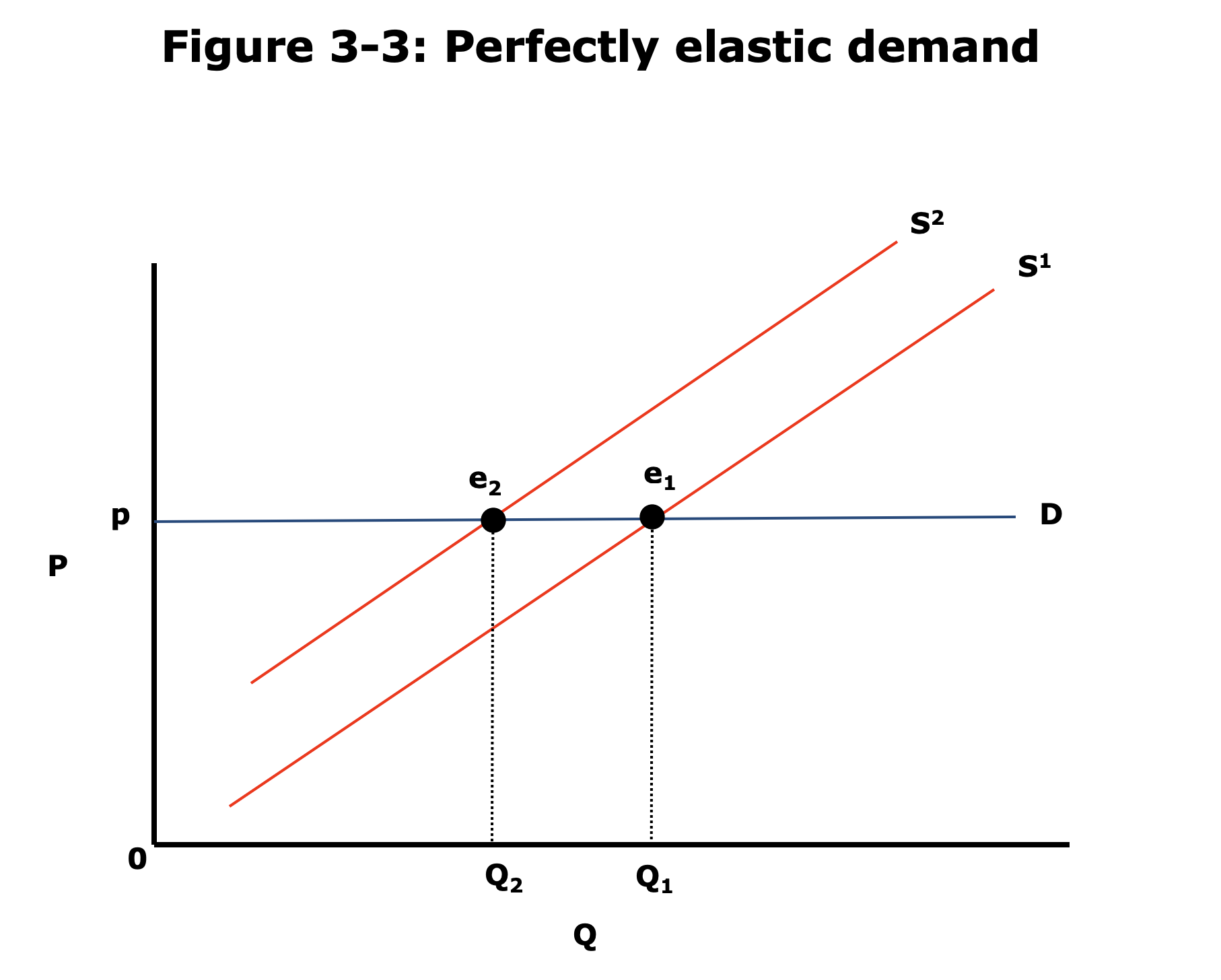
- Where consumers don't care about quantity, but only about price.
- Example: There are infinitely good substitutes.
  - E.g. Candy. Orbit and Eclipse. McDonalds and Burger King.
  - If price of Orbit increases people would buy Eclipse.
  - If there is a supply shock, price could not change, only qty supplied would change.
Peek ahead about Producer theory:
- Revenue R = Q * P (unit: $)
- (dR/R)/(dP/P) = (dR/dP) * (P/R) = Q(1+E)*P/R = (1+E)
- If Elasticity > -1, producer benefits by raising price.
  - But then why isn't price always 0 or infinity? coming up next lectures.
Difficult to measure elasticities because of causation/correlation problem.
However, this data may be important to determine govt. policies.

We assume all consumer behaviour comes from Utility Maximisation.
Three steps:
- Assumptions:
  - Completeness: Can always pick which one I like more between A & B.
  - Transitivity: If A > B, B > C then A > C.
  - Non-Satiation: More is always better!
- Utility Functions.
- Budget constraints.
Indifference curves:
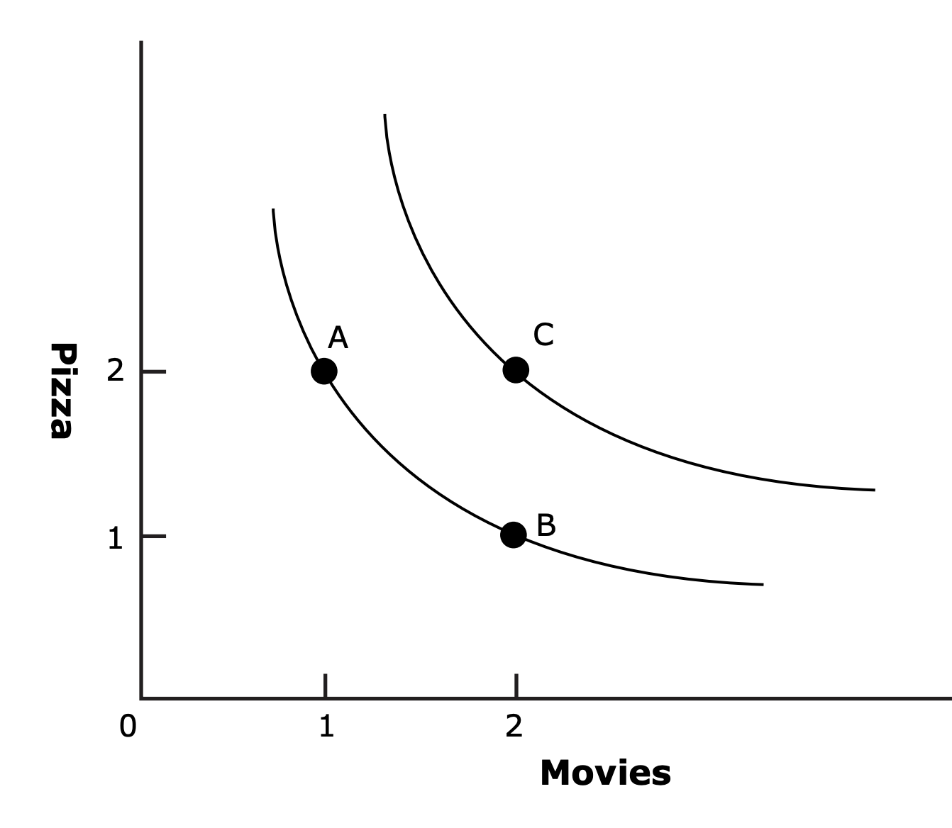
Utility: Mathematical representation of preferences.
- U(x, y) => value doesn't mean anything, only relative ranking does.
- We assume d^2 U/d(X^2) <= 0 (diminishing marginal utility)
Link between Utility and Preference maps?
- Marginal rate of substitution.
  - U(x, y) = 0 => ∂U/∂x dx + ∂U/∂y dy = 0 => dy/dx = -(∂U/∂x)/(∂U/∂y)
  - We always have diminishing marginal rate of substitution.

Assuming for now that income = budget. (No savings.)
- Good enough assumption for typical Americans.
Budget constraint: Straight line on graph (y = Sum (P_i * X_i))
Slope of the line will be (-ve of price ratio) (-P_1/P_2)
- This slope is called Marginal Rate of Transformation
Opportunity Cost
- Oppertunity cost is the value of the forgone alternative.
Maximising Utility subject to Budget Constraint
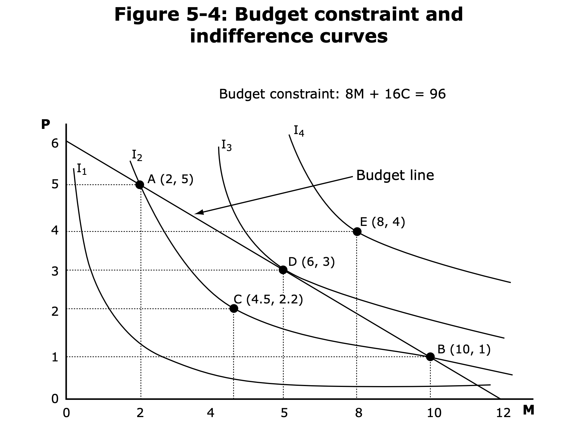
- Maximising Utility is equivalent to choosing furthest out indifference curve on the budget line.
- Indifference curve will be tangent to the budget constraint!
- The slope of the indifference curve = slope of the budget constraint!
- Marginal rate of substitution = Marginal rate of transformation!
- - (∂U/∂x_1) / (∂U/∂x_2) = - P_1 / P_2
- (Marginal) Benefit = (Marginal) Costs
- (∂U/∂x_1)/P_1 = (∂U/∂x_2)/P_2
- If this is not true, we can shift optimal point towards where we have more benefit!
- Corner solutions possible where the slopes will not be equal!
Government can affect consumption of goods through taxation.
- Or it can also use psychology to affect consumption. (Called Nudge in behavioural economics. Check out book called Nudge.)