Lecture 4
2023-04-01
MIT OCW 14.01SC L4 - Preferences and Utility
MIT OCW 14.01SC - Lec 4 (Youtube)
- So far: Overview of market, supply and demand curves.
- Now: Taking a step back and understanding where supply and demand curves come from.
- Starting with demand curve and consumer preferences. (First half of the course)
- Consumer Behaviour - Utility Maximisation
- Basically we assume all consumer behaviour comes from Utility Maximisation.
- Consumer Preferences + Budget Constriant
- What bundle of goods makes consumers best off?
- Typically we will think about two goods (because two-dimensional graphs).
- Three steps:
- Assumptions about preferences. (Axioms.)
- Translate the assumptions into mathematical function. (Utility function.)
- Budget constraints.
- Today's lecture: No budget constraints.
- Unconstrained Preferences.
- Three preference assumptions:
- Completeness: When comparing two bundles of goods, we prefer one or the other. Can't say "I'm not sure."
- Transitivity: If I prefer A > B and B > C then I prefer A > C.
- Non-satiation: (Most controversial?) More is always better. There may be diminishing returns but we will assume something > nothing.
- Indifference Curves – Preference maps (graphical representation).
- Example: Buy pizza or see movies?
- Consider 3 choices:
- 2 pizzas and 1 movie (A)
- 1 pizza and 2 movies (B)
- 2 pizzas and 2 movies (C)
- Let's say we're indifferent between A & B, but we prefer C over A or B.
- Indifference curves:
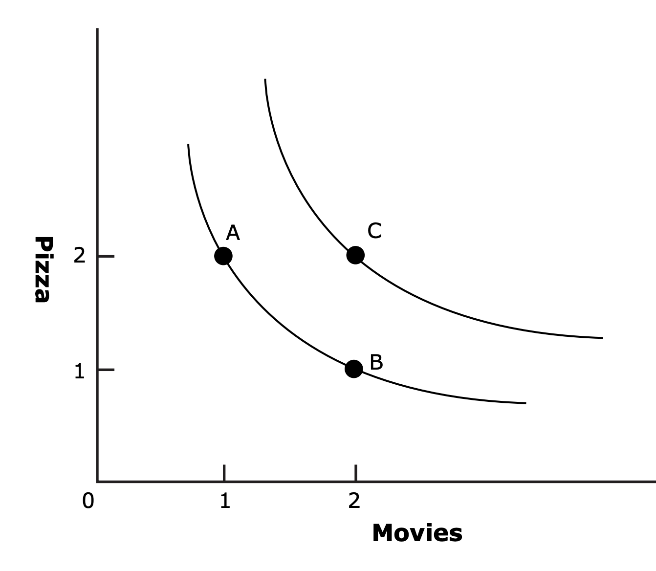
- A curve showing all possible combinations of consumption along which an individual is indifferent.
- 4 Key properties of indiffernce curves.
- Consumers prefer higher indifference curves. (From non-satiation assumption.)
- Indifferent curves are always downward sloping. (From non-satiation assumption.)
- Indifference curves cannot cross.
- Completion implies => No more than one indifference curves through a point.
- Next step: Utility.
- Mathematical representation of preference.
- Cannot tell absolute value of happiness, only useful for relative ranking.
- Example: Assume for P pizzas and M movies, utility
U = sqrt(P * M) - Marginal Utility (Key Concept!): How utility changes with each unit of input. (Derivative of utility function).
- Assume diminishing marginal utility.
marginal utility = dU/dx_i,d^2 U / d(X_i)^2 < 0
- Link between Utility and Preference maps?
- Marginal rate of substitution.
- Technically slope of indifference curve.
U(x, y) = 0=>∂U/∂x dx + ∂U/∂y dy = 0=>dy/dx = -(∂U/∂x)/(∂U/∂y)- How many Y (pizzas) are you willing to trade off for one X (movie)
- We always have diminishing marginal rate of substitution.
- Increasing diminishing marginal rate of substitution would mean an indifference curve concave to the origin.
- That wouldn't make sense. If you're willing to give up 1 Pizza for getting 1 movie, why would you give up 2 pizzas the next time to get 1 more movie? (* TODO: how to prove this formally?)
- Marginal rate of substitution.